Data and package

library(raster)
library(SingleCellExperiment)
library(scater)
library(plyr)
library(ggplot2)
library(pheatmap)
library(ggthemes)
library(RColorBrewer)
library(spatstat)
library(gridExtra)
library(ggpubr)
library(spatstat)
source("functions/image_analysis_function.R")

mibi.sce <- readRDS("../../sc-targeted-proteomics/data/mibi.sce_withDR.rds")
colnames(mibi.sce) <- paste(mibi.sce$SampleID, mibi.sce$cellLabelInImage, sep = "_")

mibi.sce$cellTypes <- ifelse(as.character(mibi.sce$immune_group) != "not immune",
                             as.character(mibi.sce$immune_group),
                             as.character(mibi.sce$tumor_group))

mibi.sce$cellTypes_group <- ifelse(as.character(mibi.sce$immune_group) != "not immune",
                                   "Micro-environment",
                                   "Tumour")



selected_chanel_mibi <- rownames(mibi.sce)[rowData(mibi.sce)$is_protein == 1]


tiff_name_list <- list.files("../../sc-targeted-proteomics/data/TNBC_shareCellData/", pattern = ".tiff")
tiff_name_list <- tiff_name_list[-24]

# color for mibi cell types
cellTypes_group_mibi_color <- tableau_color_pal("Tableau 10")(length(unique(mibi.sce$cellTypes_group)))
cellTypes_group_mibi_color <- c(cellTypes_group_mibi_color, "black")
names(cellTypes_group_mibi_color) <- c(unique(mibi.sce$cellTypes_group), "Background")

cellTypes_mibi_color <- tableau_color_pal("Classic 20")(length(unique(mibi.sce$cellTypes)))
cellTypes_mibi_color <- c(cellTypes_mibi_color, "black")
names(cellTypes_mibi_color) <- c(unique(mibi.sce$cellTypes), "Background")

common_protein <- c("CD3", "CD68", "HLA-DR", "CD45")

ot_rbind_list <- list()
for (s in 1:length(tiff_name_list)) {
  
  
  str_name <- paste("../../sc-targeted-proteomics/data/TNBC_shareCellData/", tiff_name_list[s], sep = "")
  
  sample_id <- as.numeric(gsub("p", "", gsub("_labeledcellData.tiff", "", tiff_name_list[s])))
  
  print(sample_id)
  
  p_sce <- mibi.sce[, mibi.sce$SampleID == sample_id]
  p_sce <- p_sce[rowData(p_sce)$is_protein == 1, ]
  exprsMat <- assay(p_sce, "mibi_exprs")
  
  
  # Optimal transport results
  
  epith_ot <- read.csv(paste0("../../sc-targeted-proteomics/OT/data/mibi_exprs_ot_pred_mat_epith/pred_res_mat_all_patient_", sample_id, ".csv"), row.names = 1)
  
  epith_ot <- as.matrix(epith_ot)
  
  
  
  tcells_ot <- read.csv(paste0("../../sc-targeted-proteomics/OT/data/mibi_exprs_ot_pred_mat_tcells/pred_res_mat_all_patient_", sample_id, ".csv"), row.names = 1)
  
  tcells_ot <- as.matrix(tcells_ot)
  
  
  
  
  rownames(epith_ot)[rownames(epith_ot) == "HLADR"] <- "HLA-DR"
  rownames(tcells_ot)[rownames(tcells_ot) == "HLADR"] <- "HLA-DR"
  


  
  ot_rbind <- rbind((epith_ot), 
                    (tcells_ot[!rownames(tcells_ot) %in% common_protein,]))
  
  ot_rbind <- t(apply(ot_rbind, 1, scale))
  
  colnames(ot_rbind) <- colnames(exprsMat)
  ot_rbind_list[[s]] <- ot_rbind
  
  
}

ot_rbind_list <- do.call(cbind, ot_rbind_list)
saveRDS(ot_rbind_list, "output/mibi_ot_all.rds")

Clustering on imputed matrix

ot_rbind_list <- readRDS("output/mibi_ot_all.rds")

mibi.sce_filtered <- mibi.sce[, colnames(ot_rbind_list)]

altExp(mibi.sce_filtered, "OT") <- SummarizedExperiment(list(exprs = ot_rbind_list))




mibi.sce_filtered <- scater::runPCA(mibi.sce_filtered,
                                    altexp = "OT", 
                                    ncomponents = 20,
                                    exprs_values = "exprs", name = "OT_PCA")

set.seed(2020)
mibi.sce_filtered <- scater::runUMAP(mibi.sce_filtered,
                                     altexp = "OT", 
                                     exprs_values = "exprs",
                                     pca = 20,
                                     scale = FALSE,
                                     n_neighbors = 20,
                                     name = "OT_UMAP")


# g <- scran::buildKNNGraph(mibi.sce_filtered, k = 50, use.dimred = "OT_PCA")
# clust <- igraph::cluster_louvain(g)$membership
# table(clust)

g <- scran::buildKNNGraph(mibi.sce_filtered, k = 50, use.dimred = "OT_PCA")
clust <- igraph::cluster_louvain(g)$membership
table(clust)

## clust
##     1     2     3     4     5     6     7     8     9    10    11    12    13 
##  4110 12520 16729 18822  1002 11641 11937  8758  1874  1541  3846 11122  1967 
##    14    15    16    17    18    19    20    21    22    23    24    25 
##  9738 13221  1327 13087   422 22752  6523  8367  3470  8181   722  3999

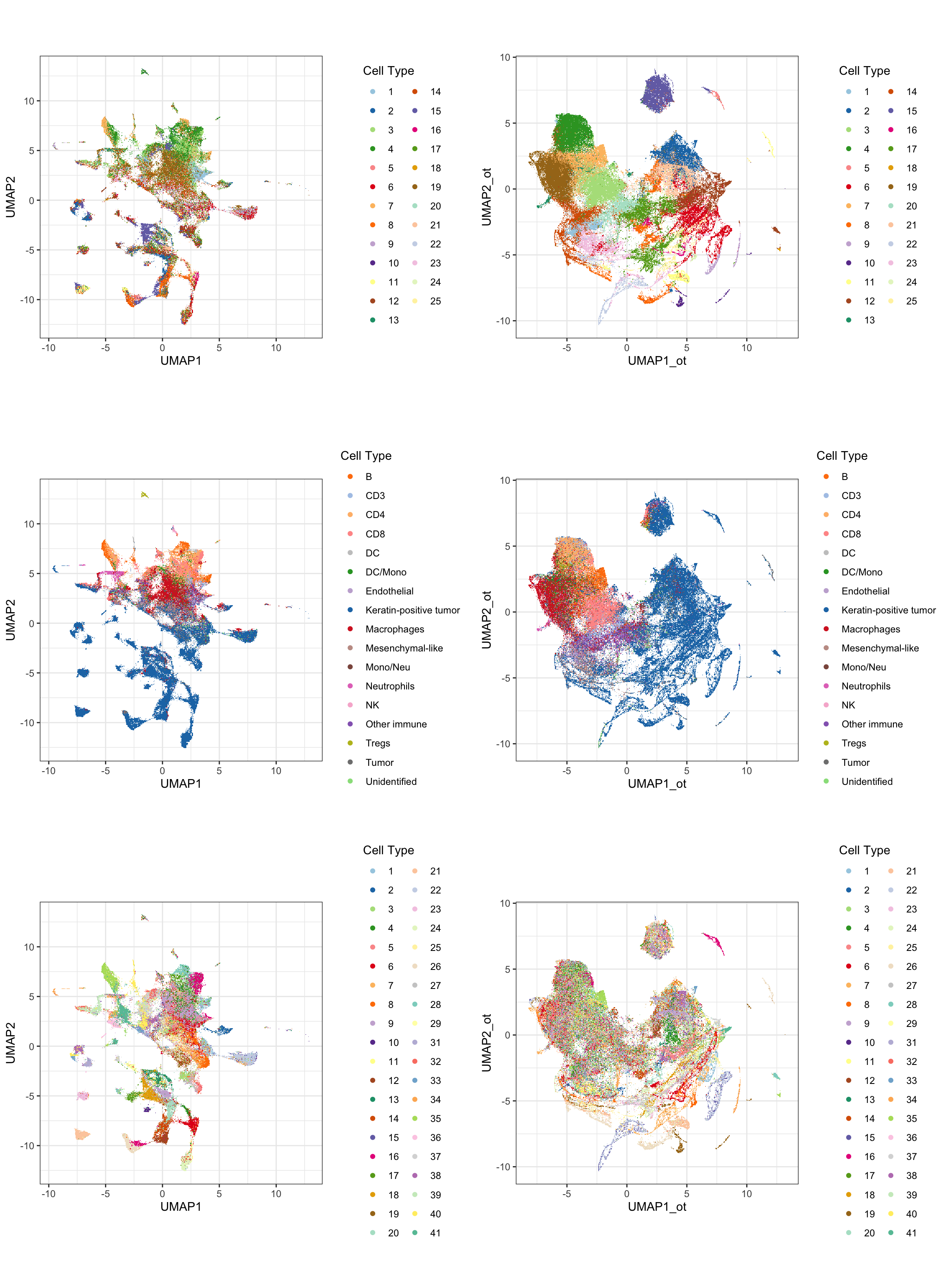
mibi.sce_filtered$ot_cluster <- as.factor(clust)

df_toPlot <- data.frame(colData(mibi.sce_filtered))

cellTypes_color_cluster <- c(RColorBrewer::brewer.pal(12, "Paired"),
                             RColorBrewer::brewer.pal(7, "Dark2"),
                             RColorBrewer::brewer.pal(8, "Pastel2"),
                             RColorBrewer::brewer.pal(12, "Set3"),
                             RColorBrewer::brewer.pal(8, "Set2"))

umap_mibi <- reducedDim(mibi.sce_filtered, "OT_UMAP")

df_toPlot$UMAP1_ot <- umap_mibi[, 1]
df_toPlot$UMAP2_ot <- umap_mibi[, 2]

umap <- reducedDim(mibi.sce_filtered, "UMAP")

df_toPlot$UMAP1 <- umap[, 1]
df_toPlot$UMAP2 <- umap[, 2]

library(scattermore)
g1 <- ggplot(df_toPlot, aes(x = UMAP1, y = UMAP2, color = ot_cluster)) + 
  geom_scattermore() +
  theme_bw() +
  theme(aspect.ratio = 1) +
  scale_color_manual(values = cellTypes_color_cluster) +
  labs(color = "Cell Type")


g2 <- ggplot(df_toPlot, aes(x = UMAP1, y = UMAP2, color = cellTypes)) + 
  geom_scattermore() +
  theme_bw() +
  theme(aspect.ratio = 1) +
  scale_color_manual(values = cellTypes_mibi_color) +
  labs(color = "Cell Type")


g3 <- ggplot(df_toPlot, aes(x = UMAP1, y = UMAP2, color = factor(SampleID))) + 
  geom_scattermore() +
  theme_bw() +
  theme(aspect.ratio = 1) +
  scale_color_manual(values = cellTypes_color_cluster) +
  labs(color = "Cell Type")



g4 <- ggplot(df_toPlot, aes(x = UMAP1_ot, y = UMAP2_ot, color = ot_cluster)) + 
  geom_scattermore() +
  theme_bw() +
  theme(aspect.ratio = 1) +
  scale_color_manual(values = cellTypes_color_cluster) +
  labs(color = "Cell Type")

g5 <- ggplot(df_toPlot, aes(x = UMAP1_ot, y = UMAP2_ot, color = cellTypes)) + 
  geom_scattermore() +
  theme_bw() +
  theme(aspect.ratio = 1) +
  scale_color_manual(values = cellTypes_mibi_color) +
  labs(color = "Cell Type")

g6 <- ggplot(df_toPlot, aes(x = UMAP1_ot, y = UMAP2_ot, color = factor(SampleID))) + 
  geom_scattermore() +
  theme_bw() +
  theme(aspect.ratio = 1) +
  scale_color_manual(values = cellTypes_color_cluster) +
  labs(color = "Cell Type")


ggarrange(g1, g4, 
          g2, g5,
          g3, g6, ncol = 2, nrow = 3, align = "hv")

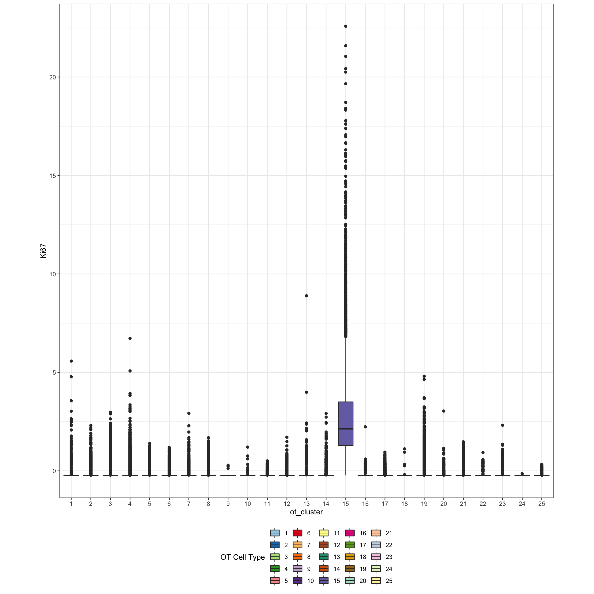
exprsMat <- assay(mibi.sce_filtered, "mibi_exprs")
ggplot(df_toPlot, aes(x = ot_cluster, y = exprsMat["Ki67", ], fill = ot_cluster)) + 
  geom_boxplot() +
  theme_bw() +
  theme(aspect.ratio = 1, legend.position = "bottom") +
  scale_fill_manual(values = cellTypes_color_cluster) +
  labs(fill = "OT Cell Type") +
  ylab("Ki67")

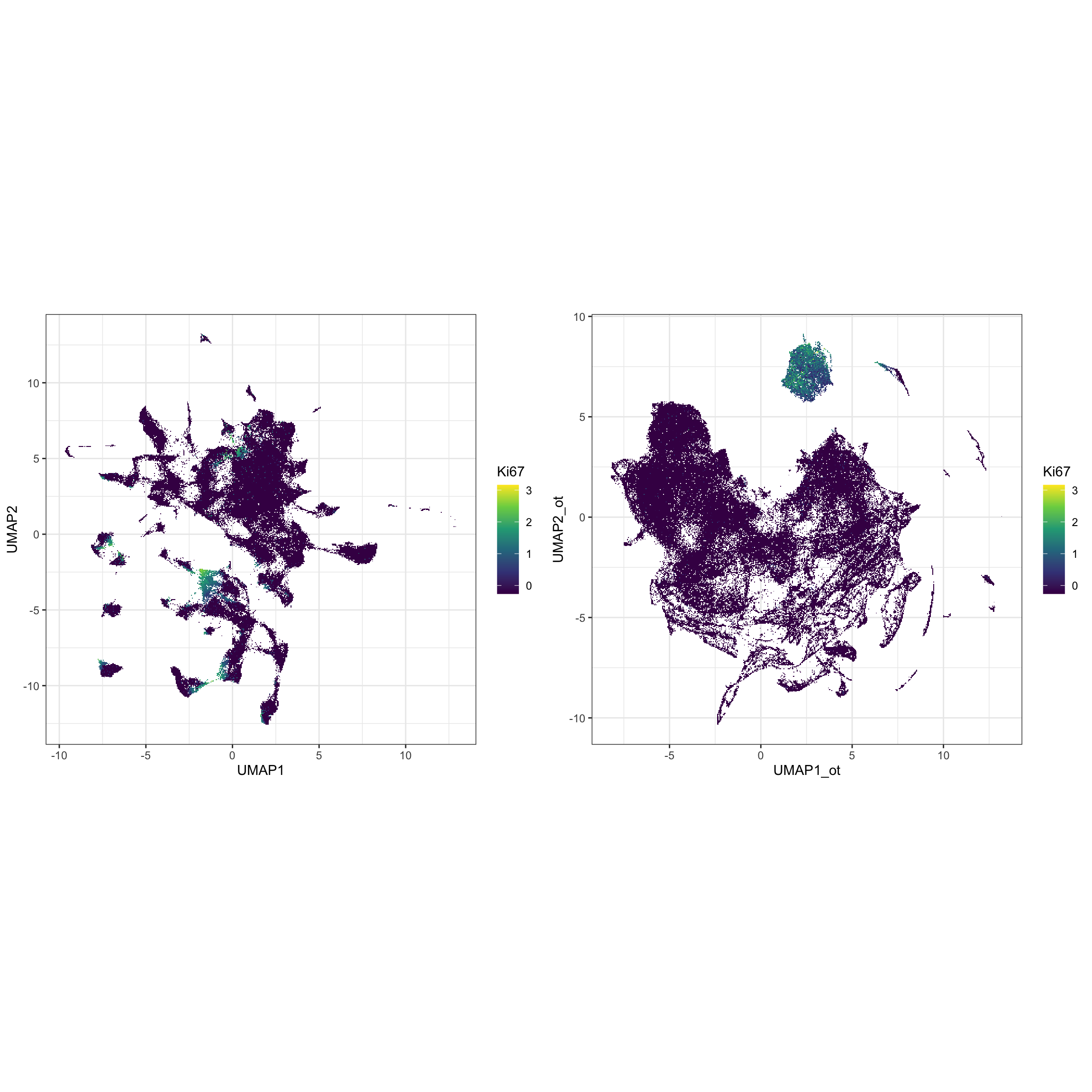
g2 <- ggplot(df_toPlot, aes(x = UMAP1_ot, y = UMAP2_ot, color = log(exprsMat["Ki67", ] + 1))) + 
  geom_scattermore() +
  theme_bw() +
  theme(aspect.ratio = 1) +
  scale_color_viridis_c() +
  labs(color = "Ki67")

g1 <- ggplot(df_toPlot, aes(x = UMAP1, y = UMAP2, color = log(exprsMat["Ki67", ] + 1))) + 
  geom_scattermore() +
  theme_bw() +
  theme(aspect.ratio = 1) +
  scale_color_viridis_c() +
  labs(color = "Ki67")

ggarrange(g1, g2, ncol = 2, nrow = 1, align = "hv")

Survival Analysis

library(survival)
library(survminer)

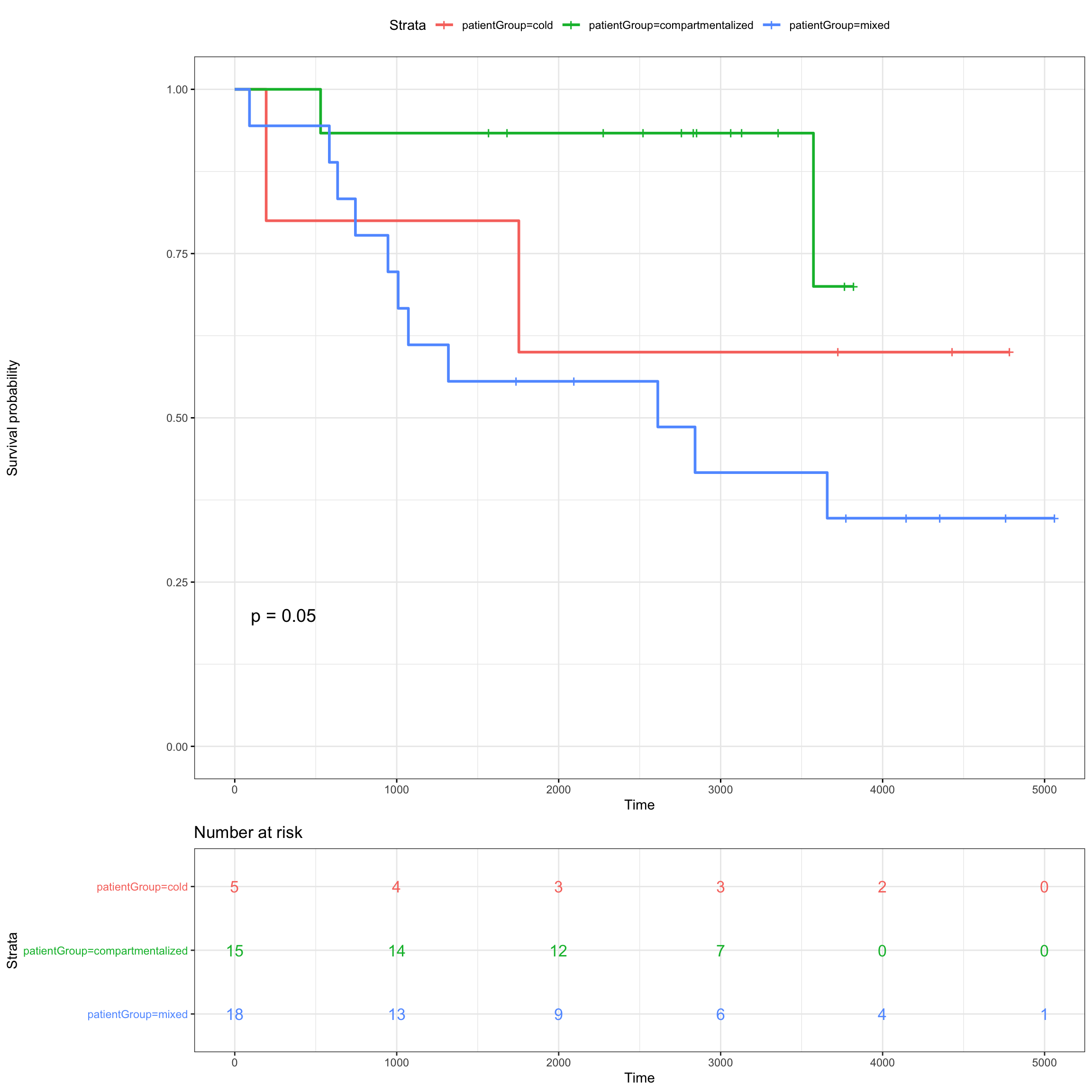
cold <- c(24, 26, 15, 22, 19, 25)
mixed <- c(13, 39, 29, 17, 23, 1, 33, 12, 27, 8, 2, 38, 20, 7, 14, 11, 21, 31, 18)
compart <- c(35, 28, 16, 37, 40, 4, 41, 36, 3, 5, 34, 32, 6, 9, 10)


mibi.sce_filtered$patientGroup <- NA
mibi.sce_filtered$patientGroup[mibi.sce_filtered$SampleID %in% mixed] <- "mixed"
mibi.sce_filtered$patientGroup[mibi.sce_filtered$SampleID %in% compart] <- "compartmentalized"
mibi.sce_filtered$patientGroup[mibi.sce_filtered$SampleID %in% cold] <- "cold"

meta_patients <- unique(data.frame(colData(mibi.sce_filtered)[, c("SampleID", "patientGroup", "Survival_days_capped_2016.1.1", "Censored", "GRADE", "STAGE", "AGE_AT_DX", "TIL_score")]))
meta_patients$STAGE <- substring(as.character(meta_patients$STAGE), 1, 1)
meta_patients$STAGE[meta_patients$STAGE %in% c(3, 4)] <- c("3_4")
meta_patients$Censoring <- 1 - meta_patients$Censored

meta_patients <- meta_patients[!is.na(meta_patients$Survival_days_capped_2016.1.1), ]
dim(meta_patients)

## [1] 38  9

colnames(meta_patients)[3] <- "SurvivalDays"
dim(meta_patients)

## [1] 38  9

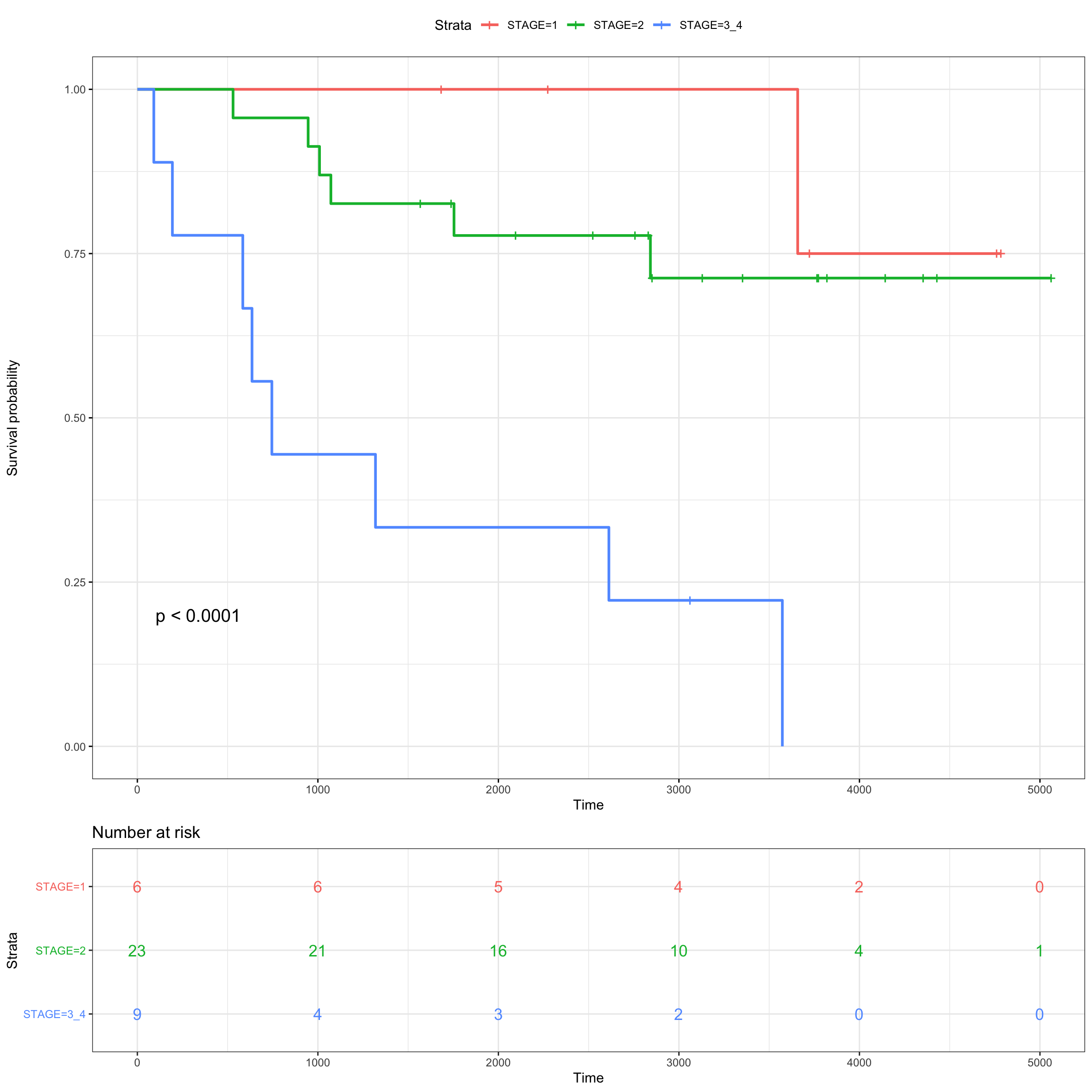
fit_stage <- survfit( Surv(SurvivalDays, Censoring) ~ STAGE,
                 data = meta_patients)



ggsurvplot(fit_stage, data = meta_patients,
           # conf.int = TRUE,
           risk.table = TRUE, risk.table.col="strata",
           ggtheme = theme_bw(),
           pval = TRUE)

fit_patientGroup <- survfit( Surv(SurvivalDays, Censoring) ~ patientGroup,
                      data = meta_patients)



ggsurvplot(fit_patientGroup, data = meta_patients,
           # conf.int = TRUE,
           risk.table = TRUE, risk.table.col = "strata",
           ggtheme = theme_bw(),
           pval = TRUE)

prop_ot <- table(mibi.sce_filtered$ot_cluster, mibi.sce_filtered$SampleID)
rownames(prop_ot) <- paste("ot_cluster_", rownames(prop_ot), sep = "")

prop_ot <- apply(prop_ot, 2, function(x) x/sum(x))

meta_patients$ki67_class <- ifelse(prop_ot[15, ][as.character(meta_patients$SampleID)] > 0.06, 
                                         "High", "Low")
meta_patients$ki67_class <- factor(meta_patients$ki67_class,
                                         levels = c("Low", "High"))
table(meta_patients$ki67_class)

## 
##  Low High 
##   23   15

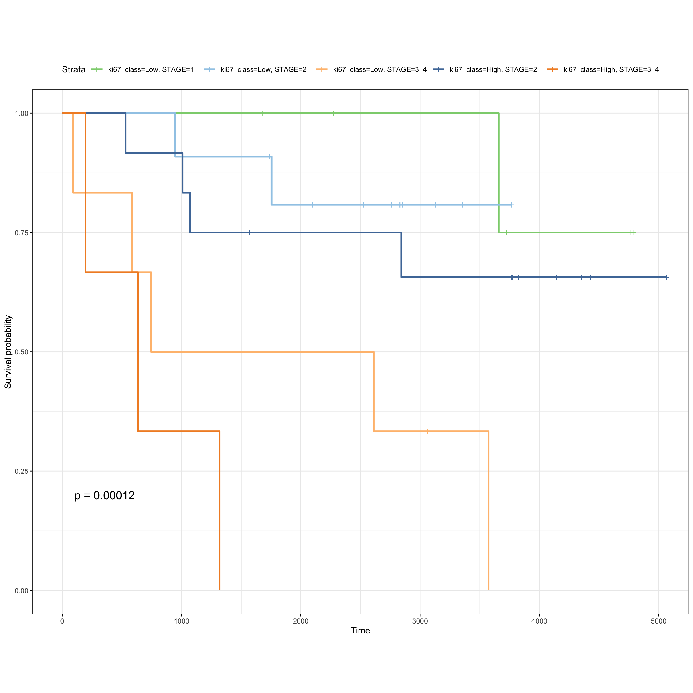
fit_ki67 <- survfit( Surv(SurvivalDays, Censoring) ~ ki67_class + STAGE,
                 data = meta_patients )

ggsurvplot(fit_ki67, data = meta_patients,
           ggtheme = theme_bw() +   theme(aspect.ratio = 0.8),
           palette = tableau_color_pal("Tableau 20")(6)[c(6, 2, 4, 1, 3)],
           pval = TRUE)

Session Information

sessionInfo()

## R Under development (unstable) (2020-03-25 r78063)
## Platform: x86_64-apple-darwin15.6.0 (64-bit)
## Running under: macOS Catalina 10.15.4
## 
## Matrix products: default
## BLAS:   /Library/Frameworks/R.framework/Versions/4.0/Resources/lib/libRblas.0.dylib
## LAPACK: /Library/Frameworks/R.framework/Versions/4.0/Resources/lib/libRlapack.dylib
## 
## locale:
## [1] en_AU.UTF-8/en_AU.UTF-8/en_AU.UTF-8/C/en_AU.UTF-8/en_AU.UTF-8
## 
## attached base packages:
## [1] parallel  stats4    stats     graphics  grDevices utils     datasets 
## [8] methods   base     
## 
## other attached packages:
##  [1] survminer_0.4.6             survival_3.1-12            
##  [3] scattermore_0.6             ggpubr_0.2.5               
##  [5] magrittr_1.5                gridExtra_2.3              
##  [7] spatstat_1.64-1             rpart_4.1-15               
##  [9] nlme_3.1-145                spatstat.data_1.4-3        
## [11] RColorBrewer_1.1-2          ggthemes_4.2.0             
## [13] pheatmap_1.0.12             plyr_1.8.6                 
## [15] scater_1.15.29              ggplot2_3.3.0              
## [17] SingleCellExperiment_1.9.3  SummarizedExperiment_1.17.5
## [19] DelayedArray_0.13.12        matrixStats_0.56.0         
## [21] Biobase_2.47.3              GenomicRanges_1.39.3       
## [23] GenomeInfoDb_1.23.16        IRanges_2.21.8             
## [25] S4Vectors_0.25.15           BiocGenerics_0.33.3        
## [27] raster_3.1-5                sp_1.4-1                   
## 
## loaded via a namespace (and not attached):
##  [1] ggbeeswarm_0.6.0         colorspace_1.4-1         ggsignif_0.6.0          
##  [4] deldir_0.1-25            ellipsis_0.3.0           XVector_0.27.2          
##  [7] BiocNeighbors_1.5.2      farver_2.0.3             RSpectra_0.16-0         
## [10] fansi_0.4.1              codetools_0.2-16         splines_4.0.0           
## [13] knitr_1.28               polyclip_1.10-0          broom_0.5.5             
## [16] km.ci_0.5-2              uwot_0.1.8               compiler_4.0.0          
## [19] dqrng_0.2.1              backports_1.1.6          assertthat_0.2.1        
## [22] Matrix_1.2-18            limma_3.43.5             cli_2.0.2               
## [25] BiocSingular_1.3.2       htmltools_0.4.0          tools_4.0.0             
## [28] rsvd_1.0.3               igraph_1.2.5             gtable_0.3.0            
## [31] glue_1.4.0               GenomeInfoDbData_1.2.2   dplyr_0.8.5             
## [34] Rcpp_1.0.4.6             vctrs_0.2.4              DelayedMatrixStats_1.9.1
## [37] xfun_0.12                stringr_1.4.0            lifecycle_0.2.0         
## [40] irlba_2.3.3              statmod_1.4.34           goftest_1.2-2           
## [43] edgeR_3.29.1             zoo_1.8-7                zlibbioc_1.33.1         
## [46] scales_1.1.0             spatstat.utils_1.17-0    yaml_2.2.1              
## [49] KMsurv_0.1-5             stringi_1.4.6            scran_1.15.26           
## [52] BiocParallel_1.21.2      rlang_0.4.5              pkgconfig_2.0.3         
## [55] bitops_1.0-6             evaluate_0.14            lattice_0.20-41         
## [58] purrr_0.3.3              tensor_1.5               labeling_0.3            
## [61] cowplot_1.0.0            tidyselect_1.0.0         RcppAnnoy_0.0.16        
## [64] R6_2.4.1                 generics_0.0.2           pillar_1.4.3            
## [67] withr_2.1.2              mgcv_1.8-31              abind_1.4-5             
## [70] RCurl_1.98-1.1           tibble_3.0.0             crayon_1.3.4            
## [73] survMisc_0.5.5           rmarkdown_2.1            viridis_0.5.1           
## [76] locfit_1.5-9.4           grid_4.0.0               data.table_1.12.8       
## [79] digest_0.6.25            xtable_1.8-4             tidyr_1.0.2             
## [82] munsell_0.5.0            beeswarm_0.2.3           viridisLite_0.3.0       
## [85] vipor_0.4.5

Integration with CyTOF

Yingxin Lin

Data and package

Clustering on imputed matrix

Survival Analysis

Session Information