Data and package
library(raster)
library(SingleCellExperiment)
library(scater)
library(plyr)
library(ggplot2)
library(pheatmap)
library(ggthemes)
library(RColorBrewer)
library(spatstat)
library(gridExtra)
library(ggpubr)
library(spatstat)
source("../R/image_analysis_functions.R")
mibi.sce <- readRDS("data/mibi.sce_withDR.rds")
colnames(mibi.sce) <- paste(mibi.sce$SampleID, mibi.sce$cellLabelInImage, sep = "_")

mibi.sce$cellTypes <- ifelse(as.character(mibi.sce$immune_group) != "not immune",
                             as.character(mibi.sce$immune_group),
                             as.character(mibi.sce$tumor_group))

mibi.sce$cellTypes_group <- ifelse(as.character(mibi.sce$immune_group) != "not immune",
                                   "Micro-environment",
                                   "Tumour")


selected_chanel_mibi <- rownames(mibi.sce)[rowData(mibi.sce)$is_protein == 1]
# color for mibi cell types
cellTypes_group_mibi_color <- tableau_color_pal("Tableau 10")(length(unique(mibi.sce$cellTypes_group)))
cellTypes_group_mibi_color <- c(cellTypes_group_mibi_color, "black")
names(cellTypes_group_mibi_color) <- c(unique(mibi.sce$cellTypes_group), "Background")

cellTypes_mibi_color <- tableau_color_pal("Classic 20")(length(unique(mibi.sce$cellTypes)))
cellTypes_mibi_color <- c(cellTypes_mibi_color, "black")
names(cellTypes_mibi_color) <- c(unique(mibi.sce$cellTypes), "Background")
tiff_name_list <- list.files("../../sc-targeted-proteomics/data/TNBC_shareCellData/", pattern = ".tiff")
tiff_name_list <- tiff_name_list[-24]

common_protein <- c("CD3", "CD68", "HLA-DR", "CD45")

ot_rbind_list <- list()
for (s in 1:length(tiff_name_list)) {


  str_name <- paste("../../sc-targeted-proteomics/data/TNBC_shareCellData/", tiff_name_list[s], sep = "")

  sample_id <- as.numeric(gsub("p", "", gsub("_labeledcellData.tiff", "", tiff_name_list[s])))

  print(sample_id)

  p_sce <- mibi.sce[, mibi.sce$SampleID == sample_id]
  p_sce <- p_sce[rowData(p_sce)$is_protein == 1, ]
  exprsMat <- assay(p_sce, "mibi_exprs")


  # Optimal transport results

  epith_ot <- read.csv(paste0("../../sc-targeted-proteomics/OT/data/mibi_exprs_ot_pred_mat_epith/pred_res_mat_all_patient_", sample_id, ".csv"), row.names = 1)

  epith_ot <- as.matrix(epith_ot)


  tcells_ot <- read.csv(paste0("../../sc-targeted-proteomics/OT/data/mibi_exprs_ot_pred_mat_tcells/pred_res_mat_all_patient_", sample_id, ".csv"), row.names = 1)

  tcells_ot <- as.matrix(tcells_ot)


  rownames(epith_ot)[rownames(epith_ot) == "HLADR"] <- "HLA-DR"
  rownames(tcells_ot)[rownames(tcells_ot) == "HLADR"] <- "HLA-DR"


  ot_rbind <- rbind((epith_ot),
                    (tcells_ot[!rownames(tcells_ot) %in% common_protein,]))

  ot_rbind <- t(apply(ot_rbind, 1, scale))

  colnames(ot_rbind) <- colnames(exprsMat)
  ot_rbind_list[[s]] <- ot_rbind


}

ot_rbind_list <- do.call(cbind, ot_rbind_list)
saveRDS(ot_rbind_list, "data/mibi_ot_all.rds")
Clustering on imputed matrix
load("data/ot_rbind_list.rda")

mibi.sce_filtered <- mibi.sce[, colnames(ot_rbind_list)]

altExp(mibi.sce_filtered, "OT") <- SummarizedExperiment(list(exprs = ot_rbind_list))


mibi.sce_filtered <- scater::runPCA(mibi.sce_filtered,
                                    altexp = "OT",
                                    ncomponents = 20,
                                    exprs_values = "exprs", name = "OT_PCA")

set.seed(2020)
mibi.sce_filtered <- scater::runUMAP(mibi.sce_filtered,
                                     altexp = "OT",
                                     exprs_values = "exprs",
                                     pca = 20,
                                     scale = FALSE,
                                     n_neighbors = 20,
                                     name = "OT_UMAP")


# g <- scran::buildKNNGraph(mibi.sce_filtered, k = 50, use.dimred = "OT_PCA")
# clust <- igraph::cluster_louvain(g)$membership
# table(clust)

g <- scran::buildKNNGraph(mibi.sce_filtered, k = 50, use.dimred = "OT_PCA")
clust <- igraph::cluster_louvain(g)$membership
table(clust)
## clust
##     1     2     3     4     5     6     7     8     9    10    11    12    13
##  4110 12520 16729 18822  1002 11641 11937  8758  1874  1541  3846 11122  1967
##    14    15    16    17    18    19    20    21    22    23    24    25
## 9738 13221 1327 13087 422 22752 6523 8367 3470 8181 722 3999mibi.sce_filtered$ot_cluster <- as.factor(clust)
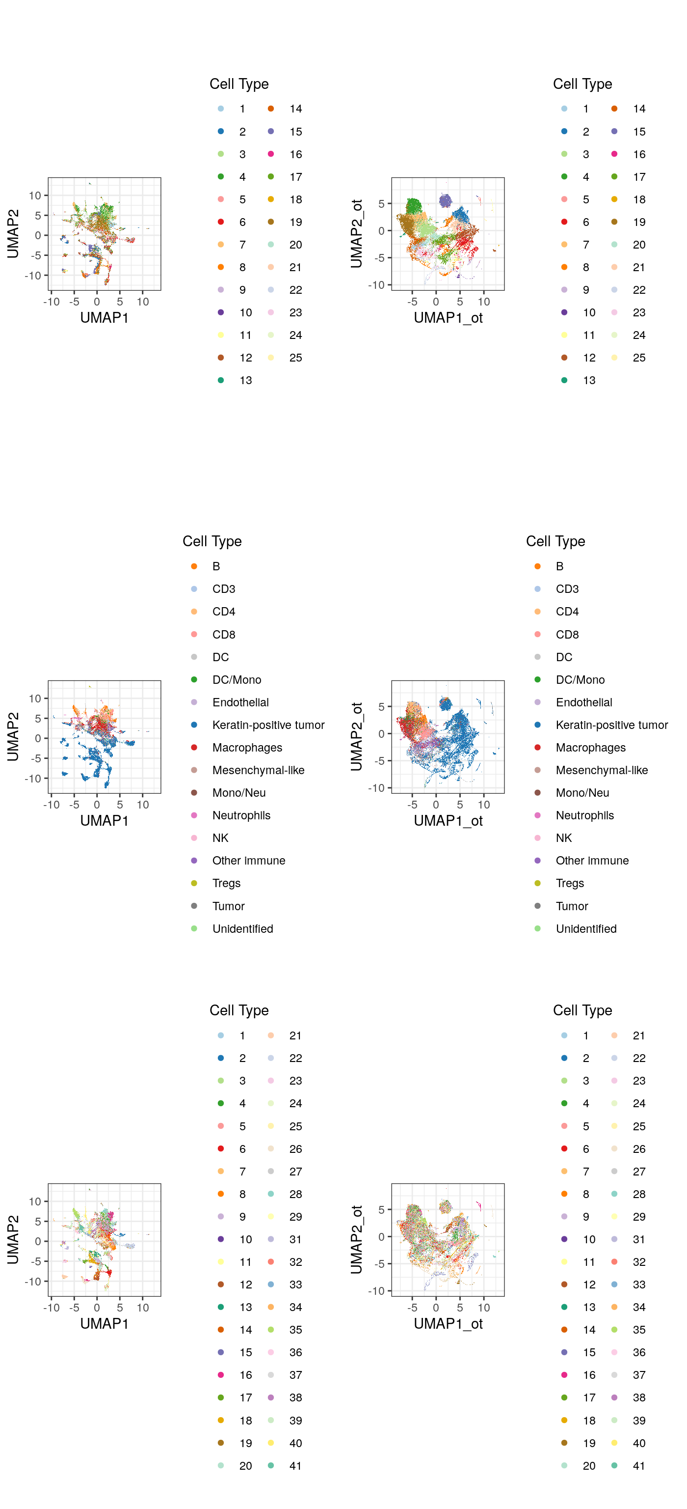
df_toPlot <- data.frame(colData(mibi.sce_filtered))

cellTypes_color_cluster <- c(RColorBrewer::brewer.pal(12, "Paired"),
                             RColorBrewer::brewer.pal(7, "Dark2"),
                             RColorBrewer::brewer.pal(8, "Pastel2"),
                             RColorBrewer::brewer.pal(12, "Set3"),
                             RColorBrewer::brewer.pal(8, "Set2"))

umap_mibi <- reducedDim(mibi.sce_filtered, "OT_UMAP")

df_toPlot$UMAP1_ot <- umap_mibi[, 1]
df_toPlot$UMAP2_ot <- umap_mibi[, 2]

umap <- reducedDim(mibi.sce_filtered, "UMAP")

df_toPlot$UMAP1 <- umap[, 1]
df_toPlot$UMAP2 <- umap[, 2]

library(scattermore)
g1 <- ggplot(df_toPlot, aes(x = UMAP1, y = UMAP2, color = ot_cluster)) +
  geom_scattermore() +
  theme_bw() +
  theme(aspect.ratio = 1) +
  scale_color_manual(values = cellTypes_color_cluster) +
  labs(color = "Cell Type")


g2 <- ggplot(df_toPlot, aes(x = UMAP1, y = UMAP2, color = cellTypes)) +
  geom_scattermore() +
  theme_bw() +
  theme(aspect.ratio = 1) +
  scale_color_manual(values = cellTypes_mibi_color) +
  labs(color = "Cell Type")


g3 <- ggplot(df_toPlot, aes(x = UMAP1, y = UMAP2, color = factor(SampleID))) +
  geom_scattermore() +
  theme_bw() +
  theme(aspect.ratio = 1) +
  scale_color_manual(values = cellTypes_color_cluster) +
  labs(color = "Cell Type")


g4 <- ggplot(df_toPlot, aes(x = UMAP1_ot, y = UMAP2_ot, color = ot_cluster)) +
  geom_scattermore() +
  theme_bw() +
  theme(aspect.ratio = 1) +
  scale_color_manual(values = cellTypes_color_cluster) +
  labs(color = "Cell Type")

g5 <- ggplot(df_toPlot, aes(x = UMAP1_ot, y = UMAP2_ot, color = cellTypes)) +
  geom_scattermore() +
  theme_bw() +
  theme(aspect.ratio = 1) +
  scale_color_manual(values = cellTypes_mibi_color) +
  labs(color = "Cell Type")

g6 <- ggplot(df_toPlot, aes(x = UMAP1_ot, y = UMAP2_ot, color = factor(SampleID))) +
  geom_scattermore() +
  theme_bw() +
  theme(aspect.ratio = 1) +
  scale_color_manual(values = cellTypes_color_cluster) +
  labs(color = "Cell Type")


ggarrange(g1, g4,
          g2, g5,
          g3, g6, ncol = 2, nrow = 3, align = "hv")
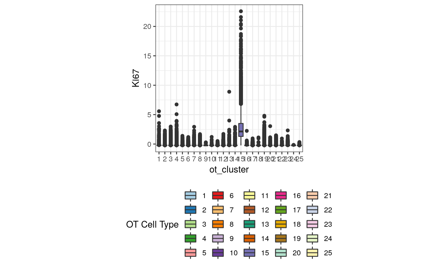
exprsMat <- assay(mibi.sce_filtered, "mibi_exprs")
ggplot(df_toPlot, aes(x = ot_cluster, y = exprsMat["Ki67", ], fill = ot_cluster)) +
  geom_boxplot() +
  theme_bw() +
  theme(aspect.ratio = 1, legend.position = "bottom") +
  scale_fill_manual(values = cellTypes_color_cluster) +
  labs(fill = "OT Cell Type") +
  ylab("Ki67")
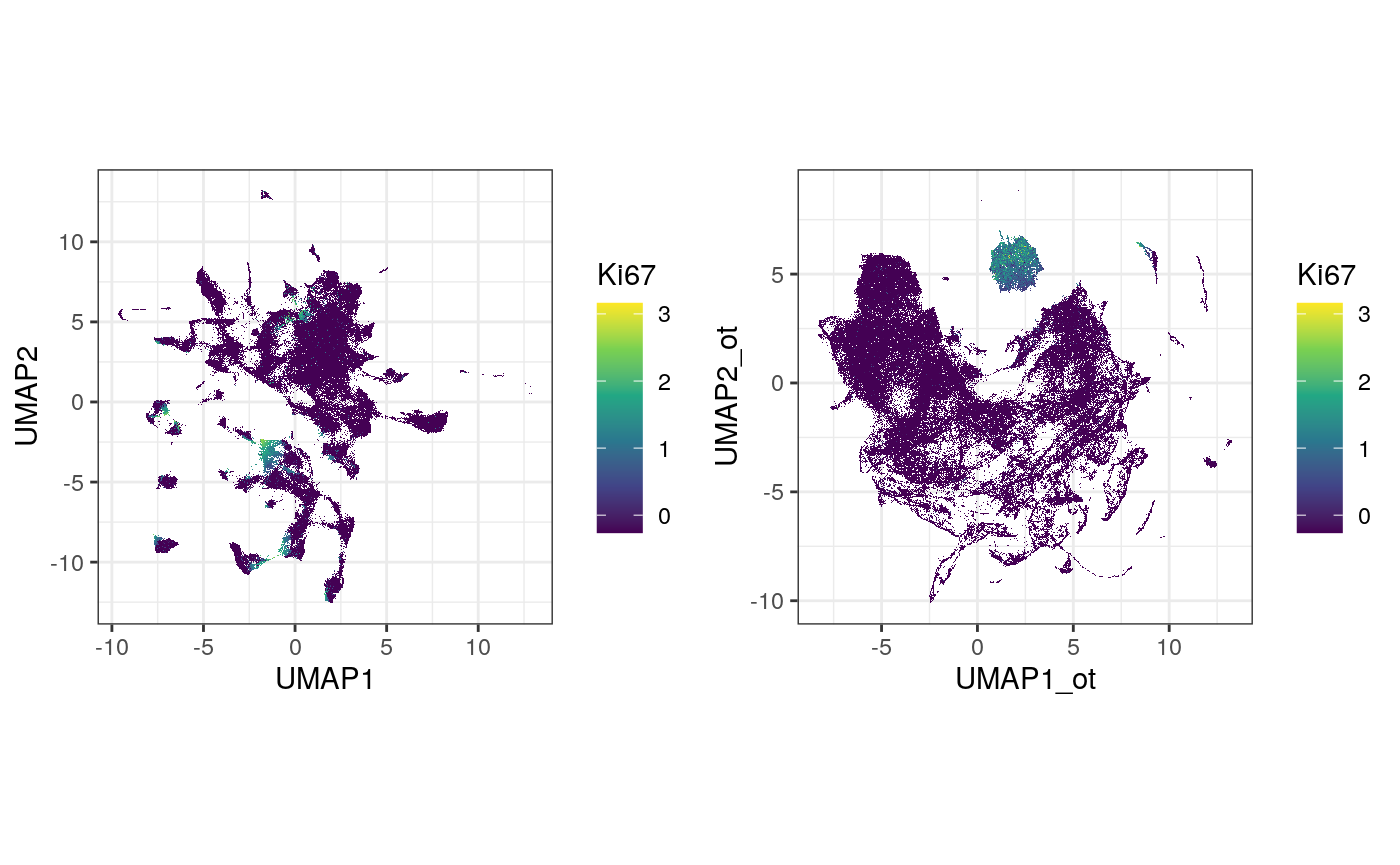
g2 <- ggplot(df_toPlot, aes(x = UMAP1_ot, y = UMAP2_ot, color = log(exprsMat["Ki67", ] + 1))) +
  geom_scattermore() +
  theme_bw() +
  theme(aspect.ratio = 1) +
  scale_color_viridis_c() +
  labs(color = "Ki67")

g1 <- ggplot(df_toPlot, aes(x = UMAP1, y = UMAP2, color = log(exprsMat["Ki67", ] + 1))) +
  geom_scattermore() +
  theme_bw() +
  theme(aspect.ratio = 1) +
  scale_color_viridis_c() +
  labs(color = "Ki67")

ggarrange(g1, g2, ncol = 2, nrow = 1, align = "hv")
Survival Analysis
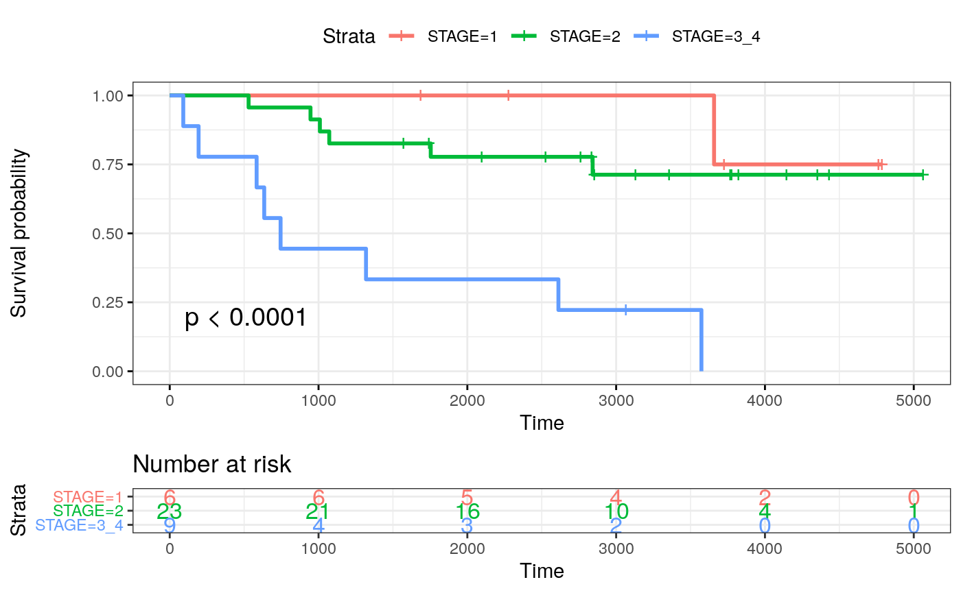
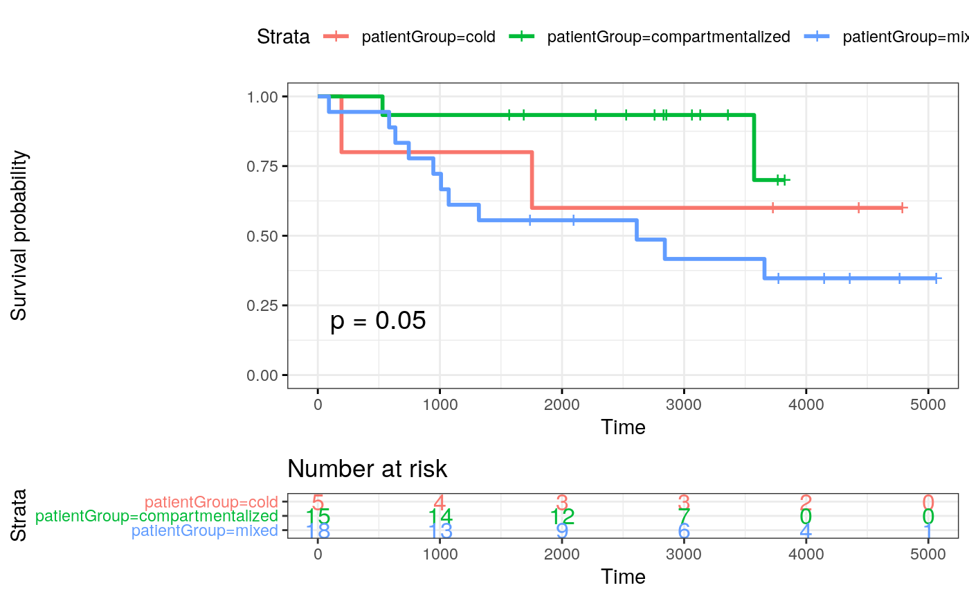
cold <- c(24, 26, 15, 22, 19, 25)
mixed <- c(13, 39, 29, 17, 23, 1, 33, 12, 27, 8, 2, 38, 20, 7, 14, 11, 21, 31, 18)
compart <- c(35, 28, 16, 37, 40, 4, 41, 36, 3, 5, 34, 32, 6, 9, 10)


mibi.sce_filtered$patientGroup <- NA
mibi.sce_filtered$patientGroup[mibi.sce_filtered$SampleID %in% mixed] <- "mixed"
mibi.sce_filtered$patientGroup[mibi.sce_filtered$SampleID %in% compart] <- "compartmentalized"
mibi.sce_filtered$patientGroup[mibi.sce_filtered$SampleID %in% cold] <- "cold"

meta_patients <- unique(data.frame(colData(mibi.sce_filtered)[, c("SampleID", "patientGroup", "Survival_days_capped_2016.1.1", "Censored", "GRADE", "STAGE", "AGE_AT_DX", "TIL_score")]))
meta_patients$STAGE <- substring(as.character(meta_patients$STAGE), 1, 1)
meta_patients$STAGE[meta_patients$STAGE %in% c(3, 4)] <- c("3_4")
meta_patients$Censoring <- 1 - meta_patients$Censored

meta_patients <- meta_patients[!is.na(meta_patients$Survival_days_capped_2016.1.1), ]
dim(meta_patients)
## [1] 38 9## [1] 38 9fit_stage <- survfit( Surv(SurvivalDays, Censoring) ~ STAGE, data = meta_patients) ggsurvplot(fit_stage, data = meta_patients, # conf.int = TRUE, risk.table = TRUE, risk.table.col="strata", ggtheme = theme_bw(), pval = TRUE)
fit_patientGroup <- survfit( Surv(SurvivalDays, Censoring) ~ patientGroup,
                      data = meta_patients)


ggsurvplot(fit_patientGroup, data = meta_patients,
           # conf.int = TRUE,
           risk.table = TRUE, risk.table.col = "strata",
           ggtheme = theme_bw(),
           pval = TRUE)
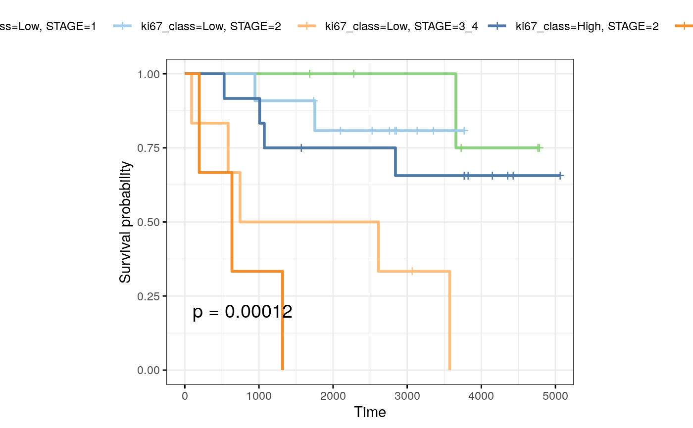
prop_ot <- table(mibi.sce_filtered$ot_cluster, mibi.sce_filtered$SampleID)
rownames(prop_ot) <- paste("ot_cluster_", rownames(prop_ot), sep = "")

prop_ot <- apply(prop_ot, 2, function(x) x/sum(x))

meta_patients$ki67_class <- ifelse(prop_ot[15, ][as.character(meta_patients$SampleID)] > 0.06,
                                         "High", "Low")
meta_patients$ki67_class <- factor(meta_patients$ki67_class,
                                         levels = c("Low", "High"))
table(meta_patients$ki67_class)
##
##  Low High
##   23   15
fit_ki67 <- survfit( Surv(SurvivalDays, Censoring) ~ ki67_class + STAGE, data = meta_patients ) ggsurvplot(fit_ki67, data = meta_patients, ggtheme = theme_bw() + theme(aspect.ratio = 0.8), palette = tableau_color_pal("Tableau 20")(6)[c(6, 2, 4, 1, 3, 5)], pval = TRUE)
Session Information
## R version 4.0.2 (2020-06-22)
## Platform: x86_64-pc-linux-gnu (64-bit)
## Running under: Ubuntu 20.04 LTS
##
## Matrix products: default
## BLAS/LAPACK: /usr/lib/x86_64-linux-gnu/openblas-openmp/libopenblasp-r0.3.8.so
##
## locale:
##  [1] LC_CTYPE=en_US.UTF-8       LC_NUMERIC=C
##  [3] LC_TIME=en_US.UTF-8        LC_COLLATE=en_US.UTF-8
##  [5] LC_MONETARY=en_US.UTF-8    LC_MESSAGES=C
##  [7] LC_PAPER=en_US.UTF-8       LC_NAME=C
##  [9] LC_ADDRESS=C               LC_TELEPHONE=C
## [11] LC_MEASUREMENT=en_US.UTF-8 LC_IDENTIFICATION=C
##
## attached base packages:
## [1] parallel  stats4    stats     graphics  grDevices utils     datasets
## [8] methods   base
##
## other attached packages:
##  [1] survminer_0.4.8             survival_3.2-3
##  [3] scattermore_0.6             ggpubr_0.4.0
##  [5] gridExtra_2.3               spatstat_1.64-1
##  [7] rpart_4.1-15                nlme_3.1-148
##  [9] spatstat.data_1.4-3         RColorBrewer_1.1-2
## [11] ggthemes_4.2.0              pheatmap_1.0.12
## [13] plyr_1.8.6                  scater_1.17.4
## [15] ggplot2_3.3.2               SingleCellExperiment_1.11.6
## [17] SummarizedExperiment_1.19.6 DelayedArray_0.15.7
## [19] matrixStats_0.56.0          Matrix_1.2-18
## [21] Biobase_2.49.0              GenomicRanges_1.41.5
## [23] GenomeInfoDb_1.25.8         IRanges_2.23.10
## [25] S4Vectors_0.27.12           BiocGenerics_0.35.4
## [27] raster_3.3-13               sp_1.4-2
##
## loaded via a namespace (and not attached):
##   [1] ggbeeswarm_0.6.0          colorspace_1.4-1
##   [3] ggsignif_0.6.0            deldir_0.1-28
##   [5] ellipsis_0.3.1            rio_0.5.16
##   [7] rprojroot_1.3-2           scuttle_0.99.11
##   [9] bluster_0.99.1            XVector_0.29.3
##  [11] BiocNeighbors_1.7.0       fs_1.5.0
##  [13] farver_2.0.3              RSpectra_0.16-0
##  [15] codetools_0.2-16          splines_4.0.2
##  [17] knitr_1.29                polyclip_1.10-0
##  [19] km.ci_0.5-2               broom_0.7.0
##  [21] uwot_0.1.8                compiler_4.0.2
##  [23] dqrng_0.2.1               backports_1.1.8
##  [25] assertthat_0.2.1          limma_3.45.9
##  [27] BiocSingular_1.5.0        htmltools_0.5.0
##  [29] tools_4.0.2               igraph_1.2.5
##  [31] rsvd_1.0.3                gtable_0.3.0
##  [33] glue_1.4.1                GenomeInfoDbData_1.2.3
##  [35] dplyr_1.0.1               Rcpp_1.0.5
##  [37] carData_3.0-4             cellranger_1.1.0
##  [39] pkgdown_1.5.1             vctrs_0.3.2
##  [41] DelayedMatrixStats_1.11.1 xfun_0.16
##  [43] stringr_1.4.0             openxlsx_4.1.5
##  [45] lifecycle_0.2.0           irlba_2.3.3
##  [47] statmod_1.4.34            rstatix_0.6.0
##  [49] goftest_1.2-2             edgeR_3.31.4
##  [51] zoo_1.8-8                 zlibbioc_1.35.0
##  [53] MASS_7.3-51.6             scales_1.1.1
##  [55] hms_0.5.3                 spatstat.utils_1.17-0
##  [57] yaml_2.2.1                curl_4.3
##  [59] memoise_1.1.0             KMsurv_0.1-5
##  [61] stringi_1.4.6             desc_1.2.0
##  [63] scran_1.17.14             zip_2.0.4
##  [65] BiocParallel_1.23.2       rlang_0.4.7
##  [67] pkgconfig_2.0.3           bitops_1.0-6
##  [69] evaluate_0.14             lattice_0.20-41
##  [71] purrr_0.3.4               tensor_1.5
##  [73] labeling_0.3              cowplot_1.0.0
##  [75] tidyselect_1.1.0          RcppAnnoy_0.0.16
##  [77] magrittr_1.5              R6_2.4.1
##  [79] generics_0.0.2            pillar_1.4.6
##  [81] haven_2.3.1               foreign_0.8-80
##  [83] withr_2.2.0               mgcv_1.8-31
##  [85] abind_1.4-5               RCurl_1.98-1.2
##  [87] tibble_3.0.3              crayon_1.3.4
##  [89] car_3.0-8                 survMisc_0.5.5
##  [91] rmarkdown_2.3             viridis_0.5.1
##  [93] locfit_1.5-9.4            grid_4.0.2
##  [95] readxl_1.3.1              data.table_1.13.0
##  [97] forcats_0.5.0             digest_0.6.25
##  [99] xtable_1.8-4              tidyr_1.1.1
## [101] munsell_0.5.0             beeswarm_0.2.3
## [103] viridisLite_0.3.0         vipor_0.4.5